Radial tree layout

The existing Diagrams.TwoD.Layout.Tree module from diagrams-contrib has been extended with a new radialLayout function, based on an algorithm by Andy Pavlo.

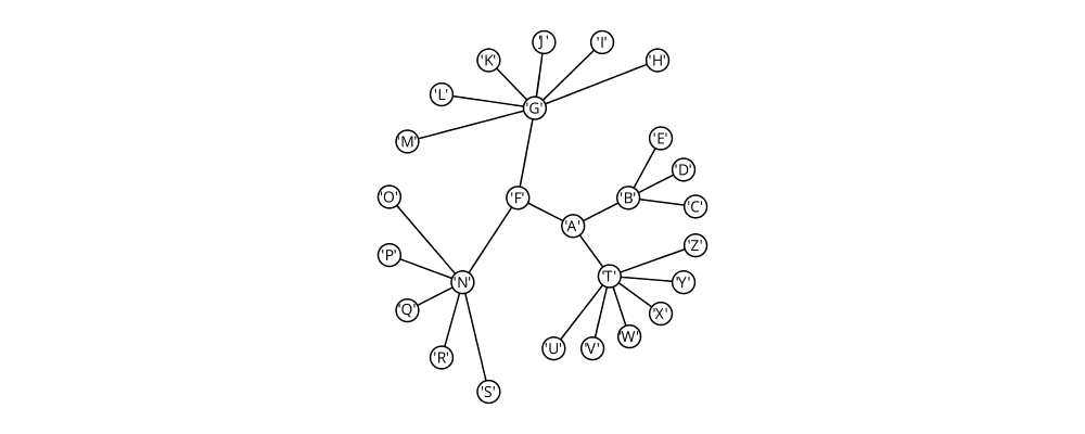
> import Diagrams.TwoD.Layout.Tree
> import Data.Tree
>
> t = Node 'A'
>     [ Node 'B' (map lf "CDE")
>     , Node 'F' [Node 'G' (map lf "HIJKLM"), Node 'N' (map lf "OPQRS")]
>     , Node 'T' (map lf "UVWXYZ")
>     ]
>   where lf x = Node x []
>
> example =
>    renderTree (\n -> (text (show n) # fontSizeG 0.5
>                             <> circle 0.5 # fc white))
>              (~~) (radialLayout t)
>    # centerXY # frame 0.5

Aligned composition

Sometimes, it is desirable to compose some diagrams according to a certain alignment, but without affecting their local origins. The composeAligned function can be used for this purpose. It takes as arguments an alignment function (such as alignT or snugL), a composition function of type [Diagram] -> Diagram, and produces a new composition function which works by first aligning the diagrams before composing them.

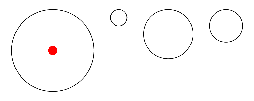
> example :: Diagram B
> example = (hsep 2 # composeAligned alignT) (map circle [5,1,3,2])
>         # showOrigin

The example above shows using hsep 2 to compose a collection of top-aligned circles. Notice how the origin of the composed diagram is still at the center of the leftmost circle, instead of at its top edge (where it would normally be placed by alignT).

Constrained layout

The new Diagrams.TwoD.Layout.Constrained module from diagrams-contrib implements basic linear constraint-based layout. As a simple example of something that would be tedious to draw without some kind of constraint solving, consider this diagram which consists of a vertical stack of circles of different sizes, along with an accompanying set of squares, such that (1) each square is constrained to lie on the same horizontal line as a circle, and (2) the squares all lie on a diagonal line.

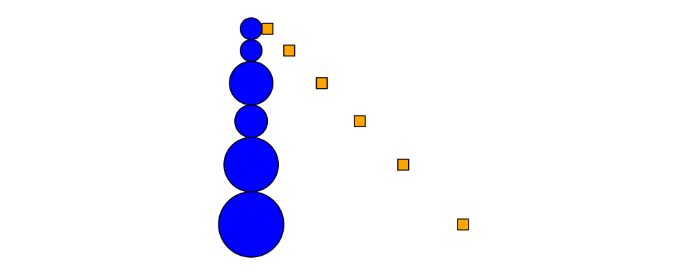
> import Diagrams.TwoD.Layout.Constrained
> import Control.Monad (zipWithM_)
>
> example :: Diagram B
> example = frame 1 $ layout $ do
>   let rs = [2,2,4,3,5,6]
>   cirs <- newDias (map circle rs # fc blue)
>   sqs  <- newDias (replicate (length rs) (square 2) # fc orange)
>   constrainWith vcat cirs
>   zipWithM_ sameY cirs sqs
>   constrainWith hcat [cirs !! 0, sqs !! 0]
>   along (direction (1 ^& (-1))) (map centerOf sqs)

See the package documentation for more examples and documentation.

Anchors

Another new module in diagrams-contrib, Diagrams.Anchors, provides a convenient interface for aligning diagrams relative to named anchor points. This can be useful, for example, when laying out diagrams composed of pieces that should "attach" to each other at various points.

We don't have an example of its use at the moment—if you play with it and create a nice example, let us know!

Boolean path operations

The new Diagrams.TwoD.Path.Boolean module from diagrams-contrib contains functions for computing boolean combinations of paths, such as union, intersection, difference, and symmetric difference.

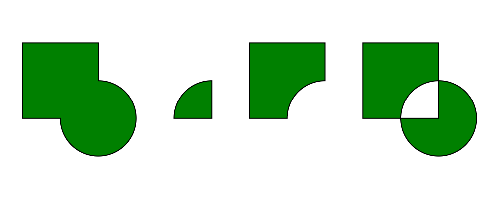
> import qualified Diagrams.TwoD.Path.Boolean as B
>
> thing1, thing2 :: Path V2 Double
> thing1 = square 1
> thing2 = circle 0.5 # translate (0.5 ^& (-0.5))
>
> example = hsep 0.5 . fc green . map strokePath $
>   [ B.union        Winding (thing1 <> thing2)
>   , B.intersection Winding thing1     thing2
>   , B.difference   Winding thing1     thing2
>   , B.exclusion    Winding thing1     thing2
>   ]

Cubic B-splines

Diagrams.CubicSpline has a new function, bspline, which creates a smooth curve (to be precise, a [uniform cubic B-spline](https://en.wikipedia.org/wiki/B-spline)) with the given points as control points. The curve begins and ends at the first and last points, and is tangent to the lines to the second-to-last control points. It does not, in general, pass through the intermediate control points.

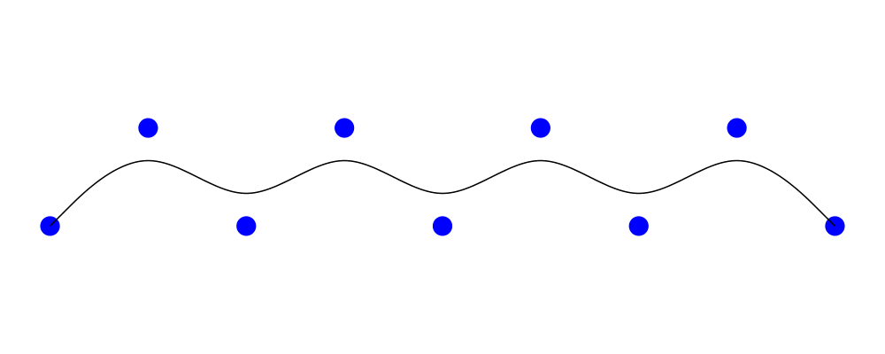
> pts = map p2 (zip [0 .. 8] (cycle [0, 1]))
> example = mconcat
>   [ bspline pts
>   , mconcat $ map (place (circle 0.1 # fc blue # lw none)) pts
>   ]

One major difference between cubicSpline and bspline is that the curves generated by cubicSpline depend on the control points in a global way—that is, changing one control point could alter the entire curve—whereas with bspline, each control point only affects a local portion of the curve.

Following composition

diagrams-contrib has a new module, Diagrams.TwoD.Path.Follow, which defines a wrapper type Following n. Following is just like Trail' Line V2, except that it has a different Monoid instance: following values are concatenated, just like regular lines, except that they are also rotated so the tangents match at the join point. In addition, they are normalized so the tangent at the start point is in the direction of the positive \(x\) axis (essentially we are considering trails equivalent up to rotation).

> import Control.Lens (ala)
> import Diagrams.TwoD.Path.Follow
>
> wibble :: Trail' Line V2 Double
> wibble = hrule 1 <> hrule 0.5 # rotateBy (1/6) <> hrule 0.5 # rotateBy (-1/6) <> a
>   where a = arc (xDir # rotateBy (-1/4)) (1/5 @@ turn)
>           # scale 0.7
>
> example =
>   [ wibble
>   , wibble
>     # replicate 5
>     # ala follow foldMap
>   ]
>   # map stroke
>   # map centerXY
>   # hsep 1
>   # frame 0.3

Notice how the above example makes use of the ala combinator from Control.Lens to automatically wrap all the Lines using follow before combining and then unwrap the result.

L-systems

The new module Diagrams.TwoD.Path.LSystem in diagrams-contrib draws L-systems described by recursive string rewriting rules, and provides a number of examples that can be used as starting points for exploration.

> import           Diagrams.TwoD.Path.LSystem
> import qualified Data.Map as M
>
> tree :: RealFloat n => Int -> TurtleState n
> tree n = lSystem n (1/18 @@ turn) (symbols "F") rules
>  where
>    rules  = M.fromList [rule 'F' "F[+>>>F]F[->>>F][>>>F]"]
>
> example = getTurtleDiagram $ tree 6

This example is already provided by the module as tree2.

XKCD colors

Randall Munroe, of xkcd fame, ran a survey to determine commonly used names for colors, and published a list of the 954 most common colors based on the results. Diagrams.Color.XKCD from diagrams-contrib provides all these color names.

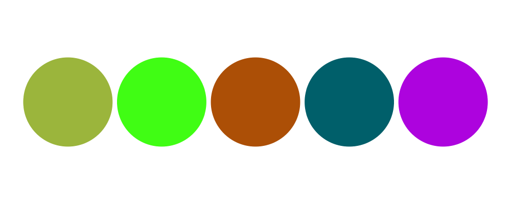
> import Diagrams.Color.XKCD
>
> colors = [booger, poisonGreen, cinnamon, petrol, vibrantPurple]
> example = hsep 0.1 (zipWith fcA colors (repeat (circle 1 # lw none)))