A reconstruction of M C Escher’s print “Square Limit”.
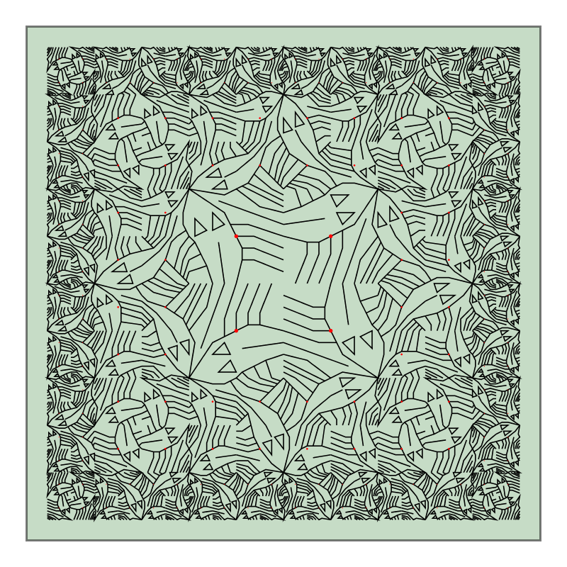
> import Diagrams.Backend.SVG.CmdLineThis is a reconstruction of M C Escher’s print “Square Limit”. It is based on the classic paper “Functional Geometry” by Peter Henderson (in Lisp and Functional Programming, 1982). But we take a slightly different approach: using lazy evaluation, we construct an infinite diagram, then prune it to some finite depth before writing out as SVG—Henderson’s code hardwired an unrolling to a particular depth.
> {-# LANGUAGE NoMonomorphismRestriction #-}
>
> import Prelude hiding (cycle)
>
> import Diagrams.Prelude
The type signatures are more specific than necessary, but perhaps easier to understand this way.
The diagram is constructed from five basic tiles: four with specific markings on, and a fifth which is blank, all \(16 \times 16\). The actual markings are defined at the end of the file.
> blank :: Diagram B
> blank = lw none $ square 16
> makeTile :: [[P2 Double]] -> Diagram B
> makeTile = showOrigin . lw thin . centerXY . mconcat . map fromVertices where> markingsP, markingsQ, markingsR, markingsS :: [[P2 Double]]Here is an algenraic datatype of pictures. Composition is by juxtaposition, which requires bounding boxes. In order to achieve this even with infinite pictures, we make all pictures the same size (\(16 \times 16\)), by scaling.
> data Picture
>   = Blank
>   | Single [[P2 Double]]
>   | Rot Picture
>   | Cycle Picture
>   | HPair Picture Picture
>   | VPair Picture Picture
>   | Quartet Picture Picture Picture Picture
>   | SkewQuartet Picture Picture Picture Picture -- left column and bottom row half size
Blank and Single correspond to the basic tiles. Rot rotates by \(90\) degrees, anticlockwise. Cycle puts together four half-size copies of a picture: unrotated at top right, and each one anticlockwise from there rotated by a further quarter turn. HPair puts two pictures side by side, and VPair one above another; each picture is scaled by a half in one dimension. Quartet puts together four pictures at half size. SkewQuartet does similarly, but in a \(2:1\) size ratio: the left column is half the width and the bottom row half the right of the right column and the top row. These maintain the invariant at all pictures are the same size.
> rot p = rotateBy (1/4) p
> cycle p = quartet (rot p) p (rot $ rot p) (rot $ rot $ rot p)
> hpair p q = scaleX (1/2) $ centerXY (p ||| q)
> vpair p q = scaleY (1/2) $ centerXY (p === q)
> quartet p q r s = scale (1/2) $ centerXY ((p ||| q) === (r ||| s))
> skewquartet p q r s = scale (1/3) $ centerXY ((scaleY 2 p ||| scale 2 q)
>                                               === (r ||| scaleX 2 s))
Folding with these operators draws a whole picture.
> drawPicture :: Picture -> Diagram B
> drawPicture Blank = blank
> drawPicture (Single m) = makeTile m
> drawPicture (Rot p) = rot (drawPicture p)
> drawPicture (Cycle p) = cycle (drawPicture p)
> drawPicture (HPair p q) = hpair (drawPicture p) (drawPicture q)
> drawPicture (VPair p q) = vpair (drawPicture p) (drawPicture q)
> drawPicture (Quartet p q r s)
>   = quartet (drawPicture p) (drawPicture q) (drawPicture r) (drawPicture s)
> drawPicture (SkewQuartet p q r s)
>   = skewquartet (drawPicture p) (drawPicture q) (drawPicture r) (drawPicture s)
Pruning with prune s p cuts off a picture p when its scale gets below \(1/s\). We keep track of the scale in \(x\) and \(y\) separately, to cope with the non-homogeneous scaling in HPair and VPair. The definition only works properly if Cycles are scaled only homogenously; that is the case in Escher’s picture.
> prune :: Double -> Picture -> Picture
> prune s p = prune' (s,s) p where
>   prune' (x,y) p | min x y < 1 = Blank -- cut off when either factor <1
>   prune' (x,y) Blank = Blank
>   prune' (x,y) (Single m) = Single m
>   prune' (x,y) (Rot p) = Rot (prune' (y,x) p)
>   prune' (x,y) (Cycle p) = Cycle (prune' (x/2,y/2) p) -- assumes x==y
>   prune' (x,y) (HPair p q) = HPair (prune' (x/2,y) p) (prune' (x/2,y) q)
>   prune' (x,y) (VPair p q) = VPair (prune' (x,y/2) p) (prune' (x,y/2) q)
>   prune' (x,y) (Quartet p q r s)
>     = Quartet (prune' x2y2 p) (prune' x2y2 q) (prune' x2y2 r) (prune' x2y2 s)
>       where x2y2 = (x/2,y/2)
>   prune' (x,y) (SkewQuartet p q r s)
>     = SkewQuartet (prune' (x3,y32) p) (prune' (x32,y32) q)
>                   (prune' (x3,y3) r) (prune' (x32,y3) s)
>       where (x3,y3,x32,y32) = (x/3,y/3,x3*2,y3*2)
Now for the construction of Escher’s Square Limit. The four basic tiles are as follows:
> fishP = Single markingsP
> fishQ = Single markingsQ
> fishR = Single markingsR
> fishS = Single markingsS
Henderson puts them together in a quartet, and cycles this:
> fishT = Quartet fishP fishQ fishR fishS
> fishU = Cycle (Rot fishQ)
This is the recursive structure of one corner of Square Limit:
> corner = SkewQuartet p q r s where
>   p = VPair p' fishT
>   p' = HPair (Rot s) p
>   q = Quartet p' q fishU s'
>   r = fishQ
>   s = HPair fishT s'
>   s' = VPair s (Rot (Rot (Rot p)))
The final picture is a cycle of these corners.
> squarelimit = Cycle corner
>
> example = drawPicture (prune 24 squarelimit) `atop` square 14.5
>         # fc darkseagreen
>         # opacity 0.5
The markings on the four basic tiles are taken from a note by Frank Buss.
> markingsP = [
>   [ (4^&4), (6^&0) ],
>   [ (0^&3), (3^&4), (0^&8), (0^&3) ],
>   [ (4^&5), (7^&6), (4^&10), (4^&5) ],
>   [ (11^&0), (10^&4), (8^&8), (4^&13), (0^&16) ],
>   [ (11^&0), (14^&2), (16^&2) ],
>   [ (10^&4), (13^&5), (16^&4) ],
>   [ (9^&6), (12^&7), (16^&6) ],
>   [ (8^&8), (12^&9), (16^&8) ],
>   [ (8^&12), (16^&10) ],
>   [ (0^&16), (6^&15), (8^&16), (12^&12), (16^&12) ],
>   [ (10^&16), (12^&14), (16^&13) ],
>   [ (12^&16), (13^&15), (16^&14) ],
>   [ (14^&16), (16^&15) ]
>   ]
> markingsQ = [
> [ (2^&0), (4^&5), (4^&7) ],
> [ (4^&0), (6^&5), (6^&7) ],
> [ (6^&0), (8^&5), (8^&8) ],
> [ (8^&0), (10^&6), (10^&9) ],
> [ (10^&0), (14^&11) ],
> [ (12^&0), (13^&4), (16^&8), (15^&10), (16^&16), (12^&10), (6^&7), (4^&7), (0^&8) ],
> [ (13^&0), (16^&6) ],
> [ (14^&0), (16^&4) ],
> [ (15^&0), (16^&2) ],
> [ (0^&10), (7^&11) ],
> [ (9^&12), (10^&10), (12^&12), (9^&12) ],
> [ (8^&15), (9^&13), (11^&15), (8^&15) ],
> [ (0^&12), (3^&13), (7^&15), (8^&16) ],
> [ (2^&16), (3^&13) ],
> [ (4^&16), (5^&14) ],
> [ (6^&16), (7^&15) ]
> ]> markingsR = [
> [ (0^&12), (1^&14) ],
> [ (0^&8), (2^&12) ],
> [ (0^&4), (5^&10) ],
> [ (0^&0), (8^&8) ],
> [ (1^&1), (4^&0) ],
> [ (2^&2), (8^&0) ],
> [ (3^&3), (8^&2), (12^&0) ],
> [ (5^&5), (12^&3), (16^&0) ],
> [ (0^&16), (2^&12), (8^&8), (14^&6), (16^&4) ],
> [ (6^&16), (11^&10), (16^&6) ],
> [ (11^&16), (12^&12), (16^&8) ],
> [ (12^&12), (16^&16) ],
> [ (13^&13), (16^&10) ],
> [ (14^&14), (16^&12) ],
> [ (15^&15), (16^&14) ]
> ]> markingsS = [
> [ (0^&0), (4^&2), (8^&2), (16^&0) ],
> [ (0^&4), (2^&1) ],
> [ (0^&6), (7^&4) ],
> [ (0^&8), (8^&6) ],
> [ (0^&10), (7^&8) ],
> [ (0^&12), (7^&10) ],
> [ (0^&14), (7^&13) ],
> [ (8^&16), (7^&13), (7^&8), (8^&6), (10^&4), (16^&0) ],
> [ (10^&16), (11^&10) ],
> [ (10^&6), (12^&4), (12^&7), (10^&6) ],
> [ (13^&7), (15^&5), (15^&8), (13^&7) ],
> [ (12^&16), (13^&13), (15^&9), (16^&8) ],
> [ (13^&13), (16^&14) ],
> [ (14^&11), (16^&12) ],
> [ (15^&9), (16^&10) ]
> ]> main = mainWith (example :: Diagram B)