Introduction

This tutorial will walk you through the basics of using the diagrams DSL to create graphics in a powerful, modular, and declarative way. There's enough here to get you started quickly; for more in-depth information, see the user manual.

This is not a Haskell tutorial (although a Haskell-tutorial-via-diagrams is a fun idea and may happen in the future). For now, we recommend Learn You a Haskell for a nice introduction to Haskell; Chapters 1-6 should give you pretty much all you need for working with diagrams.

Resources

Some resources that may be helpful to you as you learn about diagrams:

• The user manual

• The API documentation

• The diagrams-discuss mailing list

• The #diagrams IRC channel on freenode.org

Getting started

Before getting on with generating beautiful diagrams, you'll need a few things:

cabal sandbox init
cabal install diagrams

cabal exec -- ghc --make MyDiagram.hs

cabal exec bash

Philosophy

Before diving in to create some diagrams, it's worth taking a minute to explain some of the philosophy that drove many of the design decisions. (If you're particularly impatient, feel free to skip this section for now—but you might want to come back and read it later!)

• Positioning and scaling are always relative. There is never any global coordinate system to think about; everything is done relative to diagrams' local vector spaces. This is not only easier to think about, it also increases modularity and compositionality, since diagrams can always be designed without thought for the context in which they will eventually be used. Doing things this way is more work for the library and less work for the user, which is the way it should be.

• Almost everything is based around the concept of monoids (more on this later).

• The core library is as simple and elegant as possible—almost everything is built up from a very small set of primitive types and operations. One consequence is that diagrams is optimized for simplicity and flexibility rather than for speed; if you are looking to do real-time graphics generation you will probably be best served by looking elsewhere! (With that said, however, we certainly are interested in making diagrams as fast as possible without sacrificing other features, and there have been several cases of people successfully using diagrams for simple real-time graphics generation.)

Your first diagram

Create a file called DiagramsTutorial.lhs with the following contents:

> {-# LANGUAGE NoMonomorphismRestriction #-}
> {-# LANGUAGE FlexibleContexts          #-}
> {-# LANGUAGE TypeFamilies              #-}
>
> import Diagrams.Prelude
> import Diagrams.Backend.SVG.CmdLine
>
> myCircle :: Diagram B
> myCircle = circle 1
>
> main = mainWith myCircle

Turning off the Dreaded Monomorphism Restriction is quite important: if you don't, you will almost certainly run into it (and be very confused by the resulting error messages). The other two extensions are not needed for this simple example in particular, but are often required by diagrams in general, so it doesn't hurt to include them as a matter of course.

The first import statement brings into scope the entire diagrams DSL and standard library, as well as a few things from other libraries re-exported for convenience. The second import is so that we can use the SVG backend for rendering diagrams. Among other things, it provides the function mainWith, which takes a diagram as input (in this case, a circle of radius 1) and creates a command-line-driven application for rendering it.

Let's compile and run it:

$ ghc --make DiagramsTutorial.lhs
[1 of 1] Compiling Main             ( DiagramsTutorial.lhs, DiagramsTutorial.o )
Linking DiagramsTutorial ...
$ ./DiagramsTutorial -o circle.svg -w 400

If you now view circle.svg in your favorite web browser, you should see an unfilled black circle on a white background (actually, it's on a transparent background, but most browsers use white):

Be careful not to omit the -w 400 argument! This specifies that the width of the output file should be 400 units, and the height should be determined automatically. You can also specify just a height (using -h), or both a width and a height if you know the exact dimensions of the output image you want (note that the diagram will not be stretched; extra padding will be added if the aspect ratios do not match). If you do not specify a width or a height, the absolute scale of the diagram itself will be used, which in this case would be rather tiny—only 2x2.

There are several more options besides -o, -w, and -h; you can see what they are by typing ./DiagramsTutorial --help. The mainWith function is also quite a bit more general than accepting just a diagram: it can accept animations, lists of diagrams, association lists of names and diagrams, or functions producing any of the above. For more information, see the diagrams command-line creation tutorial.

A few miscellaneous notes:

• Diagrams does not require the use of literate Haskell (.lhs) files; normal .hs files work perfectly well. However, we suggest using .lhs while following diagrams tutorials, since you will be able to easily copy and paste sections of text and code from the tutorial page into your editor without reformatting it.

• The type signature on myCircle :: Diagram B is needed to inform the diagrams framework which backend you intend to use for rendering (every backend exports B as a synonym for itself). Without the type signature, you are likely to get type errors about ambiguous type variables. You can often get away with putting just one type signature on the final diagram to be rendered, and letting GHC infer the rest, though including more type signatures can also be helpful.

Attributes

Suppose we want our circle to be blue, with a thick dashed purple outline (there's no accounting for taste!). We can apply attributes to the circle diagram with the (#) operator:

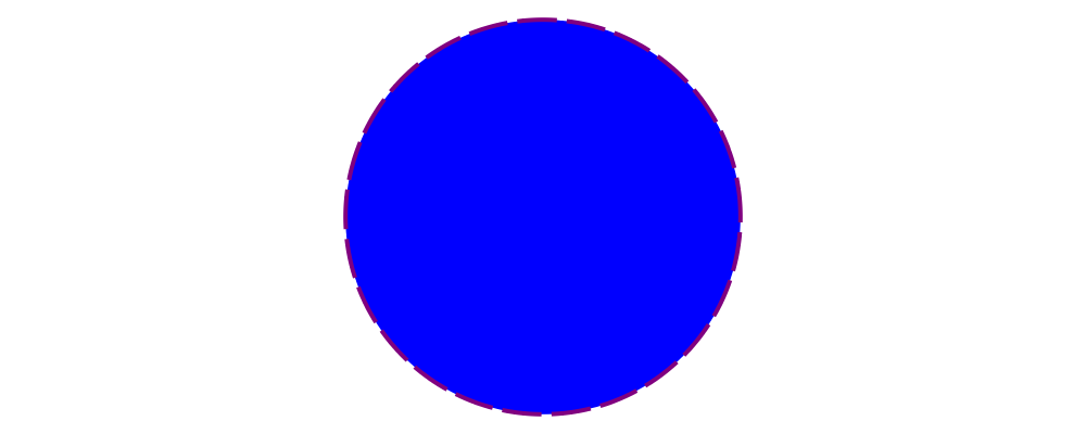
> example = circle 1 # fc blue
>                    # lw veryThick
>                    # lc purple
>                    # dashingG [0.2,0.05] 0

There's actually nothing special about the (#) operator: it's just reverse function application, that is,

> x # f = f x

Just to illustrate,

> example = dashingG [0.2,0.05] 0 . lc purple . lw veryThick . fc blue
>         $ circle 1

produces exactly the same diagram as before. So why bother with (#)? First, it's often more natural to write (and easier to read) what a diagram is first, and what it is like second. Second, (#) has a high precedence (namely, 8), making it more convenient to combine diagrams with specified attributes. For example,

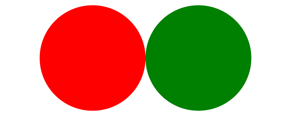
> example = circle 1 # fc red # lw none ||| circle 1 # fc green # lw none

places a red circle with no border next to a green circle with no border (we'll see more about the (|||) operator shortly). Without (#) we would have to write something with more parentheses, like

> (fc red . lw none $ circle 1) ||| (fc green . lw none $ circle 1)

For information on other standard attributes, see the Diagrams.Attributes and Diagrams.TwoD.Attributes modules.

Combining diagrams

OK, so we can draw a single circle: boring! Much of the power of the diagrams framework, of course, comes from the ability to build up complex diagrams by combining simpler ones.

Let's start with the most basic way of combining two diagrams: superimposing one diagram on top of another. We can accomplish this with atop:

> example = square 1 # fc aqua `atop` circle 1

(Incidentally, these colors are coming from the Data.Colour.Names module.)

"Putting one thing on top of another" sounds rather vague: how do we know exactly where the circle and square will end up relative to one another? To answer this question, we must introduce the fundamental notion of a local origin.

Local origins

Every diagram has a distinguished point called its local origin. Many operations on diagrams—such as atop—work somehow with respect to the local origin. atop in particular works by superimposing two diagrams so that their local origins coincide (and this point becomes the local origin of the new, combined diagram).

The showOrigin function is provided for conveniently visualizing the local origin of a diagram.

> example = circle 1 # showOrigin

Not surprisingly, the local origin of circle is at its center. So is the local origin of square. This is why square 1 `atop` circle 1 produces a square centered on a circle.

Side-by-side

Another fundamental way to combine two diagrams is by placing them next to each other. The (|||) and (===) operators let us conveniently put two diagrams next to each other in the horizontal or vertical directions, respectively. For example, horizontal:

> example = circle 1 ||| square 2

and vertical:

> example = circle 1 === square 2

The two diagrams are arranged next to each other so that their local origins are on the same horizontal or vertical line. As you can ascertain for yourself with showOrigin, the local origin of the new, combined diagram coincides with the local origin of the first diagram.

The hcat and vcat functions are provided for laying out an entire list of diagrams horizontally or vertically:

> circles = hcat (map circle [1..6])
> example = vcat (replicate 3 circles)

See also hsep and vsep for including space in between subsequent diagrams.

(|||) and (===) are actually just convenient specializations of the more general beside combinator. beside takes as arguments a vector and two diagrams, and places them next to each other "along the vector"—that is, in such a way that the vector points from the local origin of the first diagram to the local origin of the second.

> circleSqV1 = beside (r2 (1,1)) (circle 1) (square 2)
>
> circleSqV2 = beside (r2 (1,-2)) (circle 1) (square 2)
>
> example = hcat [circleSqV1, strutX 1, circleSqV2]

Notice how we use the r2 function to create a 2D vector from a pair of coordinates; see the vectors and points tutorial for more.

Envelopes

How does the diagrams library figure out how to place two diagrams "next to" each other? And what exactly does "next to" mean? There are many possible definitions of "next to" that one could imagine choosing, with varying degrees of flexibility, simplicity, and tractability. The definition of "next to" adopted by diagrams is as follows:

To place two diagrams next to each other in the direction of a vector v, place them as close as possible so that there is a separating line perpendicular to v; that is, a line perpendicular to v such that the first diagram lies completely on one side of the line and the other diagram lies completely on the other side.

There are certainly some tradeoffs in this choice. The biggest downside is that adjacent diagrams sometimes end up with undesired space in between them. For example, the two rotated ellipses in the diagram below have some space between them. (Try adding a vertical line between them with vrule and you will see why.)

> example = ell ||| ell
>   where ell = circle 1 # scaleX 0.5 # rotateBy (1/6)

However:

• This rule is very simple, in that it is easy to predict what will happen when placing two diagrams next to each other.

• It is also tractable. Every diagram carries along with it an "envelope"—a function which takes as input a vector v, and returns the minimum distance to a separating line from the local origin in the direction of v. When composing two diagrams with atop we take the pointwise maximum of their envelopes; to place two diagrams next to each other we use their envelopes to decide how to reposition their local origins before composing them with atop.

Happily, in this particular case, it is possible to place the ellipses tangent to one another (though this solution is not quite as general as one might hope):

> example = ell # snugR <> ell # snugL
>   where ell = circle 1 # scaleX 0.5 # rotateBy (1/6)

The snug class of functions use diagrams' trace (something like an embedded raytracer) rather than their envelope. (For more information, see Diagrams.TwoD.Align and the user manual section on traces.)

Transforming diagrams

As you would expect, there is a range of standard functions available for transforming diagrams, such as:

• scale (scale uniformly)

• scaleX and scaleY (scale in the X or Y axis only)

• rotate (rotate by an Angle)

• rotateBy (rotate by a fraction of a circle)

• reflectX and reflectY for reflecting along the X and Y axes

For example:

> circleRect  = circle 1 # scale 0.5 ||| square 1 # scaleX 0.3
>
> circleRect2 = circle 1 # scale 0.5 ||| square 1 # scaleX 0.3
>                                                 # rotateBy (1/6)
>                                                 # scaleX 0.5
>
> example = hcat [circleRect, strutX 1, circleRect2]

(Of course, circle 1 # scale 0.5 would be better written as just circle 0.5.)

Translation

Of course, there are also translation transformations like translate, translateX, and translateY. These operations translate a diagram within its local vector space—that is, relative to its local origin.

> example = circle 1 # translate (r2 (0.5, 0.3)) # showOrigin

As the above example shows, translating a diagram by (0.5, 0.3) is the same as moving its local origin by (-0.5, -0.3).

Since diagrams are always composed with respect to their local origins, translation can affect the way diagrams are composed.

> circleSqT   = square 1 `atop` circle 1 # translate (r2 (0.5, 0.3))
> circleSqHT  = square 1 ||| circle 1 # translate (r2 (0.5, 0.3))
> circleSqHT2 = square 1 ||| circle 1 # translate (r2 (19.5, 0.3))
>
> example = hcat [circleSqT, strutX 1, circleSqHT, strutX 1, circleSqHT2]

As circleSqHT and circleSqHT2 demonstrate, when we place a translated circle next to a square, it doesn't matter how much the circle was translated in the horizontal direction—the square and circle will always simply be placed next to each other. The vertical direction matters, though, since the local origins of the square and circle are placed on the same horizontal line.

Aligning

It's quite common to want to align some diagrams in a certain way when placing them next to one another—for example, we might want a horizontal row of diagrams aligned along their top edges. The alignment of a diagram simply refers to its position relative to its local origin, and convenient alignment functions are provided for aligning a diagram with respect to its envelope. For example, alignT translates a diagram in a vertical direction so that its local origin ends up exactly on the edge of its envelope.

> example = hrule (2 * sum sizes) === circles # centerX
>   where circles = hcat . map alignT . zipWith scale sizes
>                 $ repeat (circle 1)
>         sizes   = [2,5,4,7,1,3]

See Diagrams.TwoD.Align for other alignment combinators.

Diagrams as a monoid

As you may have already suspected if you are familiar with monoids, diagrams form a monoid under atop. This means that you can use (<>) instead of atop to superimpose two diagrams. It also means that mempty is available to construct the "empty diagram", which takes up no space and produces no output.

Quite a few other things in the diagrams standard library are also monoids (transformations, trails, paths, styles, colors, envelopes, traces...).

A worked example

As a way of exhibing a complete example and introducing some additional features of diagrams, consider trying to draw the following picture:

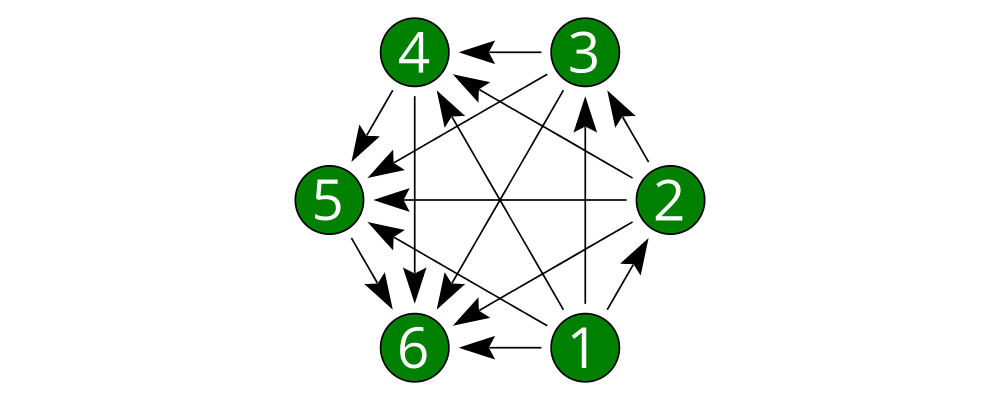
This features a hexagonal arrangement of numbered nodes, with an arrow from node \(i\) to node \(j\) whenever \(i < j\). While we're at it, we might as well make our program generic in the number of nodes, so it generates a whole family of similar diagrams.

The first thing to do is place the nodes. We can use the regPoly function to produce a regular polygon with sides of a given length. (In this case we want to hold the side length constant, rather than the radius, so that we can simply make the nodes a fixed size. To create polygons with a fixed radius as well as many other types of polygons, use the polygon function.)

> example = regPoly 6 1

However, regPoly (and most other functions for describing shapes) can be used to produce not just a diagram, but also a trail or path. Loosely speaking, trails are purely geometric, one-dimensional tracks through space, and paths are collections of trails; see the tutorial on trails and paths for a more detailed account. Trails and paths can be explicitly manipulated and computed with, and used, for example, to describe and position other diagrams. In this case, we can use the trailVertices and atPoints functions to place nodes at the vertices of the trail produced by regPoly:

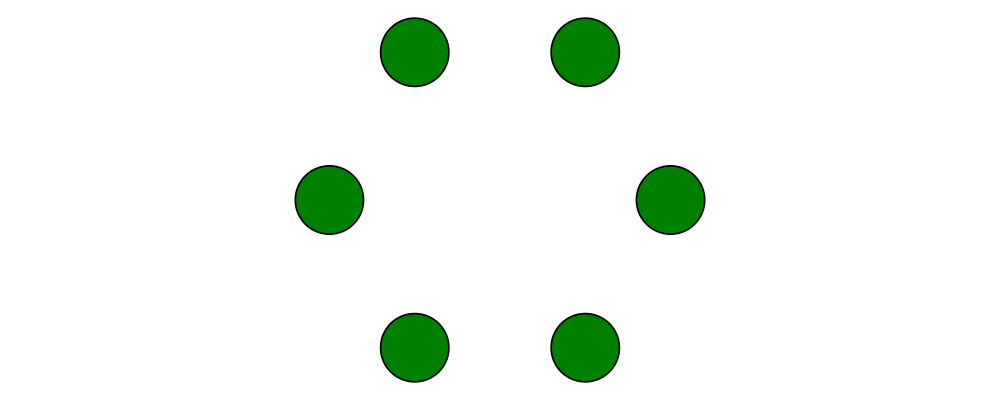
> node    = circle 0.2 # fc green
> example = atPoints (trailVertices $ regPoly 6 1) (repeat node)

As a next step, we can add text labels to the nodes. For quick and dirty text, we can use the text function provided by diagrams-lib. (For more sophisticated text support, see the SVGFonts package.) While we are at it, we also abstract over the number of nodes:

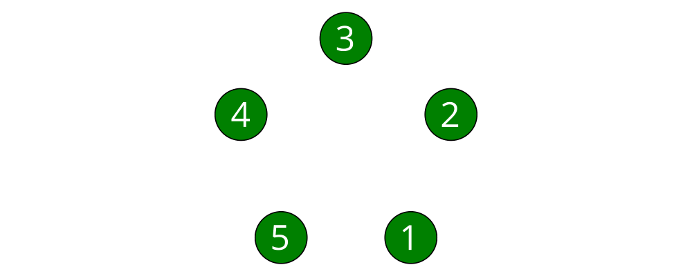
> node :: Int -> Diagram B
> node n = text (show n) # fontSizeL 0.2 # fc white <> circle 0.2 # fc green
>
> tournament :: Int -> Diagram B
> tournament n = atPoints (trailVertices $ regPoly n 1) (map node [1..n])
>
> example = tournament 5

Note the use of the type B, which is exported by every backend as a synonym for its particular backend type tag. This makes it easier to switch between backends while still giving explicit type signatures for your code: in contrast to a type like Diagram SVG which is explicitly tied to a particular backend and would have to be changed when switching to a different backend, the B in Diagram B will get instantiated to whichever backend happens to be in scope.

Our final task is to connect the nodes with arrows. First, in order to specify the parts of the diagram between which arrows should be drawn, we need to give names to the nodes, using the named function:

> node :: Int -> Diagram B
> node n = text (show n) # fontSizeL 0.2 # fc white
>       <> circle 0.2 # fc green # named n
>
> tournament :: Int -> Diagram B
> tournament n = atPoints (trailVertices $ regPoly n 1) (map node [1..n])

Note the addition of ... # named n to the circles making up the nodes. This doesn't yet change the picture in any way, but it sets us up to describe arrows between the nodes. We can use values of arbitrary type (subject to a few restrictions) as names; in this case the obvious choice is the Int values corresponding to the nodes themselves. (See the user manual section on named subdiagrams for more.)

The Diagrams.TwoD.Arrow module provides a number of tools for drawing arrows (see also the user manual section on arrows and the arrow tutorial). In this case, we can use the connectOutside function to draw an arrow between the outer edges of two named objects. Here we connect nodes 1 and 2:

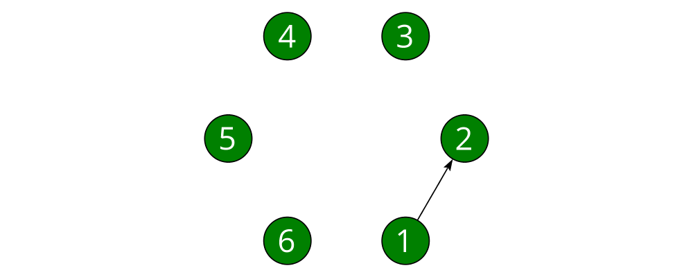
> node :: Int -> Diagram B
> node n = text (show n) # fontSizeL 0.2 # fc white
>       <> circle 0.2 # fc green # named n
>
> tournament :: Int -> Diagram B
> tournament n = atPoints (trailVertices $ regPoly n 1) (map node [1..n])
>
> example = tournament 6 # connectOutside (1 :: Int) (2 :: Int)

(The type annotations on 1 and 2 are necessary since numeric literals are polymorphic and we can use names of any type.)

This won't do, however; we want to leave some space between the nodes and the ends of the arrows, and to use a slightly larger arrowhead. Fortunately, the arrow-drawing code is highly configurable. Instead of connectOutside we can use its sibling function connectOutside' (note the prime) which takes an extra record of options controlling the way arrows are drawn. We want to override the default arrowhead size as well as specify gaps before and after the arrow, which we do as follows:

> node :: Int -> Diagram B
> node n = text (show n) # fontSizeL 0.2 # fc white
>       <> circle 0.2 # fc green # named n
>
> tournament :: Int -> Diagram B
> tournament n = atPoints (trailVertices $ regPoly n 1) (map node [1..n])
>
> example = tournament 6
>   # connectOutside' (with & gaps       .~ small
>                           & headLength .~ local 0.15
>                     )
>     (1 :: Int) (2 :: Int)

with is a convenient name for the default arguments record, and we update it using the lens library. (This pattern is common throughout diagrams; See the user manual section on optional named arguments.)

Now we simply need to call connectOutside' for each pair of nodes. applyAll, which applies a list of functions, is useful in this sort of situation.

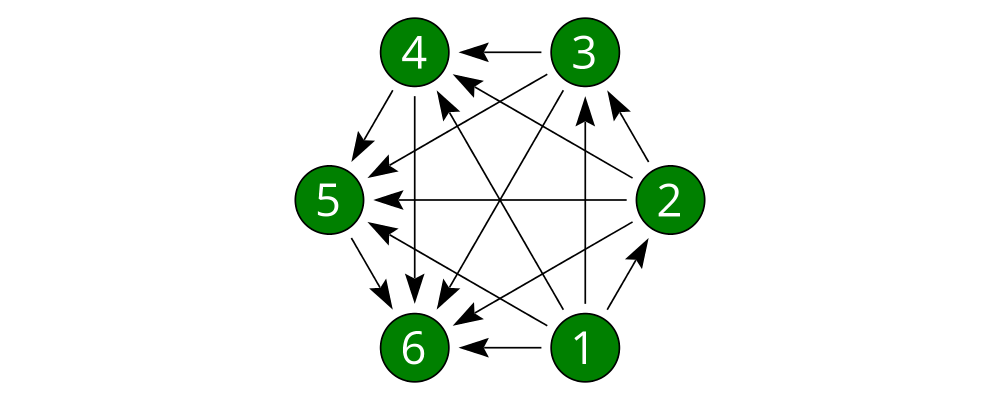
> node :: Int -> Diagram B
> node n = text (show n) # fontSizeL 0.2 # fc white
>       <> circle 0.2 # fc green # named n
>
> arrowOpts = with & gaps       .~ small
>                  & headLength .~ local 0.15
>
> tournament :: Int -> Diagram B
> tournament n = atPoints (trailVertices $ regPoly n 1) (map node [1..n])
>   # applyAll [connectOutside' arrowOpts j k | j <- [1 .. n-1], k <- [j+1 .. n]]
>
> example = tournament 6

Voilá!

Next steps

This tutorial has really only scratched the surface of what is possible! Here are pointers to some resources for learning more:

• There are other tutorials on more specific topics available. For example, there is a tutorial on working with vectors and points, one on trails and paths, one on drawing arrows between things, one on construting command-line driven interfaces, and others.

• The diagrams user manual goes into much more depth on all the topics covered in this tutorial, plus many others, and includes lots of illustrative examples. If there is anything in the manual that you find unclear, confusing, or omitted, please report it as a bug!

• The diagrams-lib API is generally well-documented; start with the documentation for Diagrams.Prelude, and then drill down from there to learn about whatever you are interested in. If there is anything in the API documentation that you find unclear or confusing, please report it as a bug as well!

• If you run into difficulty or have any questions, join the #diagrams IRC channel on freenode.org, or the diagrams-discuss mailing list.