NOTE This documentation has not yet been properly converted from its original LateX source, nor rewritten for use in the manual
We introduce a notion of polarities as a means of pre-detecting incompatibilities between candidate trees for different propositions. This optimisation is inserted between lexical selection and tree assembly. The input to this optimisation is the target semantics and the corresponding candidate trees.
This whole optimisation is based on adding polarities to the grammar. We have a set of strings which we call polarity keys, and some positive or negative integers which we call charges. Each tree in the grammar may assign a charge to some number of polarity keys. For example, here is a simple grammar that uses the polarity keys n and v.
| tree | polarity effects |
|---|---|
| s(n ↓ , v ↓ , n ↓ ) | –2n -v |
| v(hates) | +v |
| n(mary) | +n |
| n(john) | +n |
For now, these annotations are done by hand, and are based on syntactic criteria (substitution and root node categories) but one could envisage alternate criteria or an eventual means of automating the process.
The basic idea is to use the polarity keys to determine which subsets of candidate trees are incompatible with each other and rule them out. We construct a finite state automaton which uses polarity keys to pre-calculate the compatibility of sets of trees. At the end of the optimisation, we are left with an automaton, each path of which is a potentially compatible set of trees. We then preform surface realisation seperately, treating each path as a set of candidate trees.
Important note: one thing that may be confusing in this chapter is that we refer to polarities (charges) as single integers, e.g, − 2n. In reality, to account for weird stuff like atomic disjunction, we do not use simple integers, but polarities intervals, so more something like ( − 2, − 2)n! But for the most part, the intervals are zero length, and you can just think of − 2n as shorthand for ( − 2, − 2)n.
The basic process for constructing a polarity automaton is as follows:
Build a seed automaton (section {sec:seed_automaton}).
For each polarity key, elaborate the automaton with the polarity information for that key (section {sec:automaton_construction}) and minimise the automaton (section {sec:automaton_pruning}).
The above process can be thought of as a more efficient way of constructing an automaton for each polarity key, minimising said automaton, and then taking their intersection. In any case, we return everything a tuple with (1) a list of the automota that were created (2) the final automaton (3) a possibly modified input semantics. The first item is only neccesary for debugging; only the last two are important.
We construct a finite state automaton for each polarity key that is in the set of trees. It helps to imagine a table where each column corresponds to a single proposition.
gift(g) |
cost(g,x) |
high(x) |
|---|---|---|
| the gift +1np | the cost of | is high –1np |
| the present +1np | costs –1np | a lot |
| much |
Each column (proposition) has a different number of cells which corresponds to the lexical ambiguity for that proposition, more concretely, the number of candidate trees for that proposition. The {polarity automaton} describes the different ways we can traverse the table from column to column, choosing a cell to pass through at each step and accumulating polarity along the way. Each state represents the polarity at a column and each transition represents the tree we chose to get there. All transitions from one columns i to the next i + 1 that lead to the same accumulated polarity lead to the same state.
We build the columns for the polarity automaton as follows. Given a input semantics sem and a list of trees cands, we group the trees by the first literal of sem that is part of their tree semantics.
Note: this is not the same function as Tags.mapBySem! The fact that we preserve the order of the input semantics is important for our handling of multi-literal semantics and for semantic frequency sorting.
{sec:seed_automaton} We first construct a relatively trivial polarity automaton without any polarity effects. Each state except the start state corresponds to a literal in the target semantics, and the transitions to a state consist of the trees whose semantics is subsumed by that literal.
{sec:automaton_construction} {sec:automaton_intersection} The goal is to construct a polarity automaton which accounts for a given polarity key k. The basic idea is that given literals p1. . pn in the target semantics, we create a start state, calculate the states/transitions to p1 and succesively calculate the states/transitions from proposition px to px + 1 for all 1 < x < n.
The ultimate goal is to construct an automaton that accounts for multiple polarity keys. The simplest approach would be to calculate a seperate automaton for each key, prune them all and then intersect the pruned automaton together, but we can do much better than that. Since the pruned automata are generally much smaller in size, we perform an iterative intersection by using a previously pruned automaton as the skeleton for the current automaton. This is why we don’t pass any literals or candidates to the construction step; it takes them directly from the previous automaton. See also section {sec:seed_automaton} for the seed automaton that you can use when there is no “previous automaton”.
Any path through the automaton which does not lead to final polarity of zero sum can now be eliminated. We do this by stepping recursively backwards from the final states:
Lexical items with a null semantics typically correspond to functions words: complementisers “John likes to read.”, subcategorised prepositions “Mary accuses John of cheating.“
Such items need not be lexical items at all. We can exploit TAG’s support for trees with multiple anchors, by treating them as co-anchors to some primary lexical item. The English infinitival to, for example, can appear in the tree to take as s(comp(to),v(take),np ↓ ).
On the other hand, pronouns have a {zero-literal} semantics, one which is not null, but which consists only of a variable index. For example, the pronoun she in ({ex:pronoun_pol_she}) has semantics {s} and in ({ex:pronoun_pol_control}), {he} has the semantics {j}.
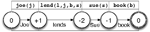
joe(j) sue(s) book(b) lend(l j b s) boring(b)
Joe lends Sue a boring book.
joe(j) book(b) lend(l j b s) boring(b)
Joe lends her a boring book.
joe(j), sue(s), leave(l,j), promise(p,j,s,l) Joe promises Sue that he would leave.
In the figure below, we compare the construction of polarity automata for ({ex:pronoun_pol_sue}, left) and ({ex:pronoun_pol_she}, right). Building an automaton for ({ex:pronoun_pol_she}) fails because {sue} is not available to cancel the negative polarities for {lends}; instead, a pronoun must be used to take its place. The problem is that the selection of a lexical items is only triggered when the construction algorithm visits one of its semantic literals. Since pronoun semantics have zero literals, they are never selected. Making pronouns visible to the construction algorithm would require us to count the indices from the input semantics. Each index refers to an entity. This entity must be “consumed” by a syntactic functor (e.g. a verb) and “provided” by a syntactic argument (e.g. a noun).
Difficulty with zero-literal semantics.
We make this explicit by annotating the semantics of the lexical input (that is the set of lexical items selected on the basis of the input semantics) with a form of polarities. Roughly, nouns provide indices1 ( + ), modifiers leave them unaffected, and verbs consume them ( − ). Predicting pronouns is then a matter of counting the indices. If the positive and negative indices cancel each other out, no pronouns are required. If there are more negative indices than positive ones, then as many pronouns are required as there are negative excess indices. In the table below, we show how the example semantics above may be annotated and how many negative excess indices result:
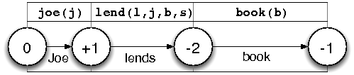
Counting surplus indices allows us to establish the number of pronouns used and thus gives us the information needed to build polarity automata. We implement this by introducing a virtual literal for negative excess index, and having that literal be realised by pronouns. Building the polarity automaton as normal yields lexical combinations with the required number of pronouns, as in figure {fig:polarity_automaton_zerolit}.
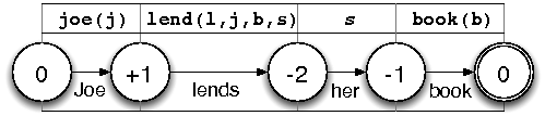
Constructing a polarity automaton with zero-literal semantics
{different_sem_annotations} The sitation is more complicated where the lexical input contains lexical items with different annotations for the same semantics. For instance, the control verb {promise} has two forms: one which solicits an infinitive as in {promise to leave}, and one which solicits a declarative clause as in {promise that he would leave}. This means two different counts of subject index {j} in ({ex:pronoun_pol_control}) : zero for the form that subcategorises for the infinitive, or one for the declarative. But to build a single automaton, these counts must be reconciled, i.e., how many virtual literals do we introduce for {j}, zero or one? The answer is to introduce enough virtual literals to satisfy the largest demand, and then use the multi-literal extension to support alternate forms with a smaller demand. To handle example ({ex:pronoun_pol_control}), we introduce one virtual literal for {j} so that the declarative form can be produced, and treat the soliciting {promise} as though its semantics includes that literal along with its regular semantics (figure {fig:polarity_automaton_zerolit_promise}). In other words, the infinitive-soliciting form is treated as if it already fulfils the role of a pronoun, and does not need one in its lexical combination.
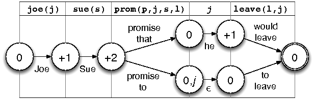
Constructing a polarity automaton with zero-literal semantics
We insert pronouns into the input semantics using the following process:
For each literal in the input semantics, establish the smallest charge for each of its semantic indices.
Cancel out the polarities for every index in the input semantics.
Compensate for any uncancelled negative polarities by an adding an additional literal to the input semantics – a pronoun – for every negative charge.
Finally, deal with the problem of lexical items who require fewer pronouns than predicted by inserting the excess pronouns in their extra literal semantics (see page {different_sem_annotations})
Automatic detection is not an optimisation in itself, but a means to make grammar development with polarities more convenient.
Our detection process looks for attributes which are defined on all subst and root nodes of the lexically selected items. Note that this should typically give you the cat and idx polarities. It is only used to give you hints about what features you may want to consider using in the graphical interface.
First the simplified explanation: we assign every tree with a − 1 charge for every category for every substitution node it has. Additionally, we assign every initial tree with a + 1 charge for the category of its root node. So for example, the tree s(n ↓ , cl ↓ , v(aime), n ↓ ) should have the following polarities: s +1, cl –1, n –2. These charges are added to any that previously been defined in the grammar.
Now what really happens: we treat automaton polarities as intervals, not as single integers! For the most part, nothing changes from the simplified explanation. Where we added a − 1 charge before, we now add a ( − 1, − 1) charge. Similarly, we where added a + 1 charge, we now add (1, 1).
So what’s the point of all this? It helps us deal with atomic disjunction. Suppose we encounter a substitution node whose category is either cl or n. What we do is add the polarities cl( − 1, 0), n( − 1, 0) which means that there are anywhere from –1 to 0 cl, and for n.
Chart sharing is based on the idea that instead of performing a seperate generation task for each automaton path, we should do single generation task, but annotate each tree with set of the automata paths it appears on. We then allow trees on the same paths to be compared only if they are on the same path
To minimise the number of states in the polarity automaton, we could also sort the literals in the target semantics by the number of corresponding lexically selected items. The idea is to delay branching as much as possible so as to mimimise the number of states in the automaton.
Let’s take a hypothetical example with two semantic literals: bar (having two trees with polarties 0 and +1). foo (having one tree with polarity –1) and If we arbitrarily explored bar before foo (no semantic sorting), the resulting automaton could look like this:
     bar     foo
(0)--+---(0)------(-1)
     |
     +---(1)------(0)
With semantic sorting, we would explore foo before bar because foo has fewer items and is less likely to branch. The resulting automaton would have fewer states.
     foo      bar
(0)-----(-1)--+---(-1)
              |
              +---(0)
The hope is that this would make the polarity automata a bit faster to build, especially considering that we are working over multiple polarity keys.
Note: we have to take care to count each literal for each lexical entry’s semantics or else the multi-literal semantic code will choke.
We can define the polarity automaton as a NFA, or a five-tuple (Q, Σ , δ, q0, qn) such that
Q is a set of states, each state being a tuple (i, e, p) where i is an integer (representing a single literal in the target semantics), e is a list of extra literals which are known by the state, and p is a polarity.
Σ is the union of the sets of candidate trees for all propositions
q0 is the start state (0, [0, 0]) which does not correspond to any propositions and is used strictly as a starting point.
qn is the final state (n, [x, y]) which corresponds to the last proposition, with polarity x ≤ 0 ≤ y.
δ is the transition function between states, which we define below.
except for predicative nouns, which like verbs, are semantic functors ↩