Kelvin, often, runs
After the lexical selection phase, we move into tree assembly. The input to this phase is the semantic formula we wish to realise, and the set of lexically selected elementary trees. Our objective is to find every derived tree that can be built from these parts and which is (i) syntactically complete, meaning it has no empty substitution sites and (ii) semantically complete, meaning that its semantics exactly matches the input semantics. Ultimately, the goal of realisation is to produce a set of strings, but this basically consists of concatenating the leaves of each derived tree.
To cope with the problem of intersective modifiers, the algorithm uses the delayed modification strategy of (TODO: citation) Realisation occurs in two chart generation phases, a substitution phase (where only TAG substitutions are performed), and an adjunction phase (likewise, TAG adjunctions only). Separating forces the realiser to only insert modifiers into syntactically complete structures. It also happens to be a very natural strategy to use with TAG because adjunction and auxiliary trees are part and parcel of the formalism. This could be seen as a potential advantage for TAG as a generation formalism (TODO: citation) .
We can think of the two phases as two successive chart generation problems fed to a generic deductive parser. For clarity, here is a more procedural description of the algorithm. We are using agenda based control mechanism common to many chart parsing algorithms, where the agenda is a data structure for storing unprocessed intermediate results. For convenience, we introduce a new data structure, called an auxiliary agenda. The auxiliary agenda is used to set aside any syntactically complete auxiliary trees found during the first phase of realisation. It is not strictly necessary, but it saves the trouble of filtering the chart afterwards. Here are the two phases in detail:
Store the lexically selected trees in the agenda, except for auxiliary trees which are devoid of substitution nodes (put these in the auxiliary agenda).
Loop: Retrieve a tree from the agenda, add it to the chart and try to combine it by substitution with trees present in the chart. Add any resulting derived tree to the agenda. Stop when the agenda is empty.
Move the chart trees to the agenda and the auxiliary agenda trees on to the chart. Discard all trees which are not syntactically complete (i.e. that still have open substitution nodes), as they will never become complete in this phase.
Loop: Retrieve a tree from the agenda, add it to the chart and try to combine it by adjunction with trees present in the chart. Add any resulting derived tree to the agenda. Stop when the agenda is empty.
The inner workings of this algorithm might be better illustrated by an example or two:
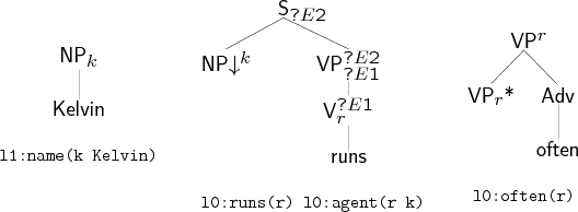
Let us start with a simple one. Suppose that the input semantics is l0:run(r) l0:agent(r k) l0:often(r) l1:name(k Kelvin). Lexical selection gives us a set of elementary trees lexicalised with the words Kelvin, often, runs. The trees for Kelvin and runs are placed on the agenda, the one for often is placed on the auxiliary agenda.
Kelvin, often, runs
We begin with the substitution phase, which consists of systematically exploring the possibility of combining two trees by substitution. Note that in the table below, the letters ‘k’, ‘r’ and ‘o’ stand for the elementary trees that correspond to Kelvin, runs and often, respectively. When the trees combine, we write, for example, ‘kr’ to mean a derived tree for Kelvin runs. We see that here, the tree for Kelvin is substituted into the one for runs, and the resulting derived tree for Kelvin runs is placed on the agenda. Trees on the agenda are processed one by one in this fashion, although in this simple example, there is only one substitution to be done. When the agenda is empty, indicating that all combinations have been tried, we prepare for the next phase.
| Combination | Agenda | Chart | AgendaA |
|---|---|---|---|
| k,r | o | ||
| r, | k | o | |
| ↓(r,k) | kr | r,k | o |
| r,k,kr | o |
All items containing an open substitution node are erased from the chart (here, the tree anchored by runs) as there is no hope that they will be made complete in this phase. The agenda is then reinitialised to the content of the chart and the chart to the content of the auxiliary agenda (here often). The adjunction phase proceeds much like the previous phase, except that now all possible adjunctions are performed. When the agenda is empty once more, the items in the chart whose semantics matches the input semantics are selected, and their strings printed out, yielding in this case the sentence Kelvin runs often.
| Combination | Agenda | Chart | Results |
|---|---|---|---|
| k,kr | o | ||
| kr | o | ||
| *(kr,o) | kro | o | |
| o | kro |
Note that the chart never changes during the adjunction phase. This is because we do not store new items onto the chart. As each tree is removed from the agenda, either we notice that it is semantically complete and save it as a result, or we perform all adjunction operations involving (i) the tree and (ii) a tree from the chart, and put any resulting derived trees back onto the agenda. The tree itself is no longer of any use and may be discarded. We will see more implications of this below, when we have more than one auxiliary tree that can adjoin into the same node.
Now, a slightly more complicated example. Here, we shall see auxiliary tree with substitution nodes, as well as a lexical selection which leads to more than one result. Our new input semantics is l1:name(k Kelvin) l0:often(r) l0:run(r k) l0:in(r i) l0:place(i Colorado) , basically the same as before with two new literals. The lexically selected trees are the same as before plus trees for in and Colorado. The trees for in, Colorado, Kelvin and runs are placed on the agenda, whereas the tree for often is placed on the auxiliary agenda.
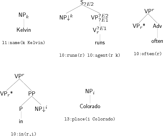
Kelvin, often, runs
Again, the substitution phase explores all possible substitutions, of which there are two: Kelvin into runs to get Kelvin runs, and Colorado into in to get in Colorado. The case of in Colorado is particularly interesting because it is a syntactically complete auxiliary tree V(V*,PP(P(in),NP(Colorado))), in the sense that it has no open substitution sites. When we produce such trees, we transfer them to the auxiliary agenda, so that they can be used during the adjunction phase.
| Combination | Agenda | Chart | AgendaA |
|---|---|---|---|
| i,c,k,r | o | ||
| c,k,r | i | o | |
| ↓(i,c) | ic,k,r | i,c | o |
| k,r | i,c | o,ic | |
| r | i,c,k | o,ic | |
| ↓(r,k) | kr | i,c,k,r | o,ic |
| i,c,k,r,kr | o,ic |
As before, all items containing an empty substitution node are erased from the chart (here, the trees anchored by runs and by in). The agenda is then reinitialised to the content of the chart and the chart to the content of the auxiliary agenda (here often and in Colorado). The adjunction phase proceeds, performing all possible adjunctions. When the agenda is empty once more, the items in the chart whose semantics matches the input semantics are selected, and their strings printed out, yielding in this case the sentences Kelvin runs often in Colorado and Kelvin runs in Colorado often.
| Combination | Agenda | Chart | Results |
|---|---|---|---|
| c,k,kr | o, ic | ||
| k,kr | o, ic | ||
| kr | o, ic | ||
| *(kr,o), *(kr,ic) | kro,kric | o, ic | |
| *(kro,ic) | kroic,kric | o, ic | |
| kric | o, ic | kroic | |
| *(kric,o) | krico | o, ic | kroic |
| o, ic | kroic, krico |
Here, we get more than one result because trees can combine in different ways (we could also get more than one result if we had an ambiguous lexical selection, but this is not the case here). Note, by the way, that the combinations here are a result of embedded adjunctions and not multiple adjunctions. The fact that supports the former but not the latter is a technical detail, and affects the number of outputs it produces (allowing for multiple adjunctions introduces more output since we cannot forbid embedded adjunctions), as well as the derivation trees for the output.